Epileptic Disorders
MENULearn to interpret voltage maps: an atlas of topographies Volume 24, numéro 2, April 2022

Illustrations
-

Figure 1
Schematic representation of post-synaptic potentials at pyramidal cells in cortical layers III-V. Excitatory postsynaptic potentials (EPSP) at the apical dendrites, far from the cell body, result in current flowing into the nerve cell. This generates negativity in the extracellular space close to the cortical surface. The return currents exit closer to the cell body and generate the corresponding positivity towards the white matter. Inhibitory postsynaptic potentials (IPSP) near the cell body force current to exit from the cell and generate positivity in the extracellular space. The return currents enter the apical dendrites and create the negativity towards the cortical surface. In both cases, the current flow creates a dipolar current flowing into the cortex with a potential distribution with negativity closer to the cortical surface and positivity closer to the white matter. This orientation of the (intracellular) current dipole and polarity distribution in the extracellular space is typical of interictal epileptiform discharges.
Figure 1 -
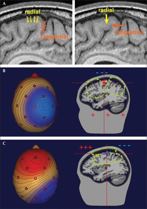
Figure 2
The orientation of the cortical generator influences the voltage topography. (A) The radial orientation of the cortical columns in the cortical convexity and the tangential orientation of the cortical columns in the wall of the sulcus illustrated on the left by small dipole current vectors summing the net current of each column. The current dipole vectors of all columns sum to an equivalent radial dipole if the activity is on the cortical convexity and to an equivalent tangential dipole if in the sulcus (thick arrows on the right). (B) A generator located at the cortical convexity. In this patch of cortex, the apical dendrites are perpendicular to the scalp, resulting in the radial direction of the current flow (illustrated on the right by the red dipole oriented downwards). The return currents in the head volume surround the generator with a small part (illustrated by the green arrows) leaving the brain remotely and entering symmetrically from the scalp above the generator to create the observed smeared scalp negativity (left). Note that this orientation leads to a large amplitude and relatively well circumscribed negativity on the scalp just over the generator. This is surrounded by widespread, low-amplitude positivity due to the volume conduction of the return currents. The positive pole is located on the opposite side of the head. The voltage distribution corresponding to this orientation is shown in the map on the left, where blue colour depicts negative potentials and red colour depicts positive potentials. (C) A generator located in the wall of a sulcus (illustrated on the right by the blue dipole pointing forward into the sulcal cortex). In this patch of cortex (marked in blue), the apical dendrites are parallel to the scalp, resulting in the tangential orientation of the current flow. The return currents in the head volume surround the generator in the opposite direction to the equivalent dipole with a small part leaving the brain over the frontal and entering over the parietal cortex (illustrated by the green arrows above the generator). This orientation leads to distinct negative and positive poles, remote from the source. In the case of a perfectly tangential dipole, as illustrated here, the poles are at a symmetric distance from the source (illustrated by the map on the left) and the source lies halfway below both poles. Note that with any non-radial (tangential or oblique) orientation, the maximum scalp negativity is not over the source, and both polarities need to be accounted for to estimate the source which is located between the negative (blue) and positive (red) poles.
Figure 2 -
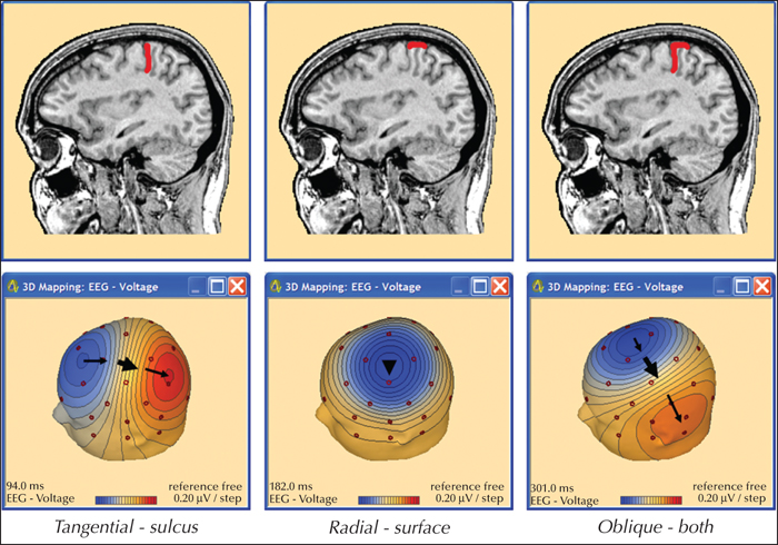
Figure 3
Voltage maps generated by cortical patches of different orientations. Voltage maps show the distribution of the negative and positive polarities on the scalp. The upper row illustrates the cortical source patches (red) of three different spikes on a sagittal MRI slice. The lower row shows the corresponding 3D voltage maps. Blue represents the negativity and red the positivity. Note the typical “dipolar” voltage distributions. The cortical source in the posterior part of the central sulcus (tangential dipole) induces two strong poles on the scalp: a negative one (anterior) and a positive one (posterior). The source of the cortical convexity (radial dipole) induces a strong negative pole on the scalp above the source while the rest of the head has a weak positivity surrounding the strong negativity with the positive pole on the opposite side of the head. When the source extends to cortical areas with different orientations (e.g. convexity and sulcus are simultaneously active), the radial and tangential dipole currents sum into an oblique equivalent dipole. In this typical case, the resulting voltage topography shows an oblique pattern with a stronger negative pole shifted away from the generating region (here towards mid-frontal) and a more remote and weaker positive pole. Thus, the negativity alone no longer indicates where the source is; the whole dipolar pattern must be interpreted [4,6]. The large arrows are above the source centre; the small arrows indicate the rule of connecting the negative to the positive pole by the shortest route. Figure from Scherg (2012) [6].
Figure 3 -
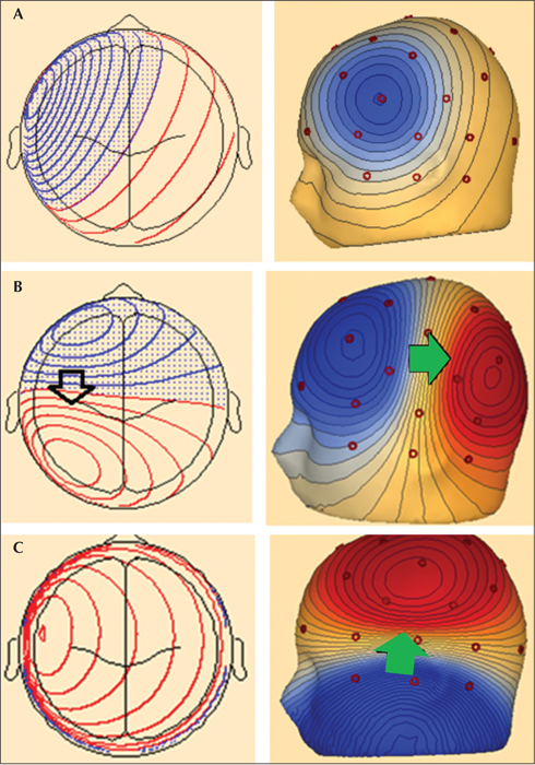
Figure 4
Reading voltage maps generated by different orientations of the cortical generators. (A) The voltage map shows a relatively well circumscribed area of negativity (maximum at FT5 electrode) surrounded by widely distributed, low-amplitude positivity that is maximal at the opposite side of the head. This distribution indicates a radial orientation of the cortical generator, hence the source is under the maximum negativity. (B). The voltage map shows a clearly defined negative pole (maximum at F3) and a clearly defined positive pole (maximum close to P3). The symmetry of the two poles suggests a tangential orientation. On the line connecting maximum negativity with maximum positivity, the source is located near the highest gradients, i.e. where the equipotential lines are closest to each other (arrow). (C) The voltage map shows a clearly defined negative pole (maximum caudal to T9) and a clearly defined positive pole (maximum close to C3). This suggests a tangential (vertical) orientation. On the line connecting maximum negativity with maximum positivity, the source is located at the highest gradient – where the equipotential lines are closest to each other (arrow). This corresponds to the basal (inferior) part of the left temporal lobe.
Figure 4 -
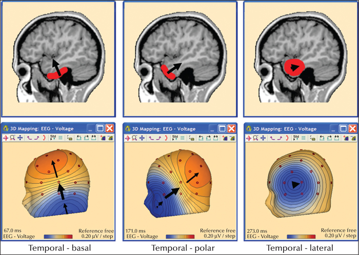
Figure 5
Typical cortical orientations in the temporal lobe. Following the rules for interpreting voltage maps, one can localize the signals to the basal (inferior), polar and lateral part of the temporal lobe. The large arrows are above the source centre; the small arrows indicate the rule of connecting the negative to the positive pole by the shortest route. Figure from Scherg (2012) [6]. Basal sources generate voltage maps with maximum negativity inferior to the edge of the recording array and positive maximum in the parasagittal area, due to the vertical orientation of the generator. Sources in the temporal pole generate topographies with maximum negativity in the anterior-inferior part of the head (around the cheek) and maximum positivity close to the midline, in the parieto-occipital area, due to the oblique orientation of this region. Sources in the lateral cortical area have radially oriented generators, resulting in maximum negativity above the source and no clearly defined positive pole (widely distributed, low-amplitude positivity surrounding the area with negative potentials).
Figure 5 -
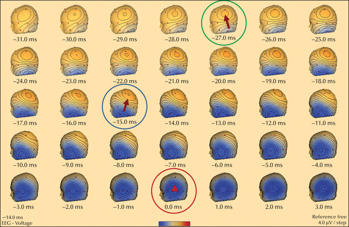
Figure 6
Sequential voltage maps during the ascending slope of a spike in the left temporal region. The red circle indicates the voltage map at the peak of the discharge (0 ms). The topography indicates a radial lateral temporal activity. However, tracing the topographic distribution back in time, one can see that the earliest onset activity (green circle, -27 ms) has a vertically oriented, tangential dipole topography that corresponds to an origin in the basal temporal region. The subsequent rotation towards a more polar dipole pattern (blue circle) indicates an increasing overlap of temporal polar over basal activity. At the peak, basal and polar activities undergo zero-crossing to revert in polarity, thus making the radial lateral activity clearly visible. This mapping sequence is a typical example of a mesio-basal spike with an origin likely in the region of the hippocampal formation, parahippocampal gyrus and/or amygdala (not visible on scalp EEG). The initial spike activities during the onset are the activities propagated from the mesial structures to the basal and/or polar surfaces of the temporal lobe before reaching the lateral temporal surface.
Figure 6 -
-
-
-
-
-
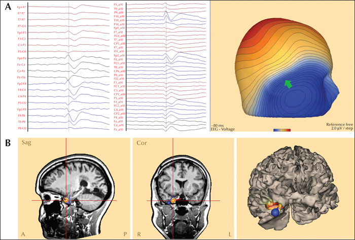
Figure 7
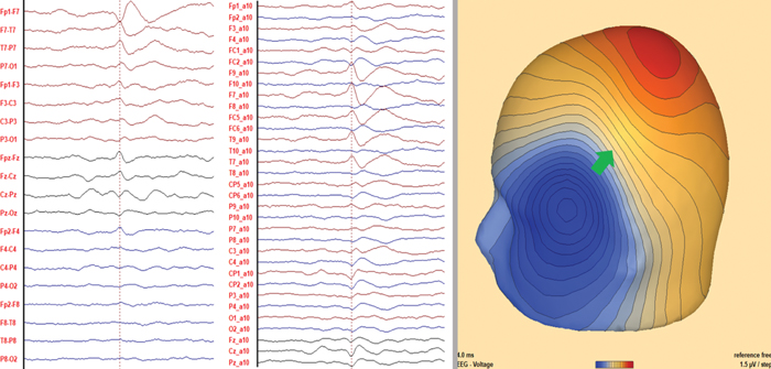
Right temporal pole (A) Maximum negativity: right anterior-inferior temporal (F8, F10). Maximum positivity: Pz. The green arrow in the voltage map shows the location of the steepest voltage gradient. This voltage distribution and the oblique orientation are typical of sources in the polar-basal region of the temporal lobe. (B) Equivalent current dipole model (first two images) and distributed source model (third image) indicate a source in the polar-basal part of the right temporal lobe. Red dipole: spike onset. Blue dipole: spike peak. The third image shows a three-dimensional image of the brain (seen from the front and right), showing the distributed source model (maximum in red) and the dipole models. MRI showed hippocampal sclerosis. The patient underwent right-sided amygdalo-hippocampectomy; the pathology showed hippocampal sclerosis and the patient achieved Engel Class 1 at 24 months after operation.
Figure 7 -
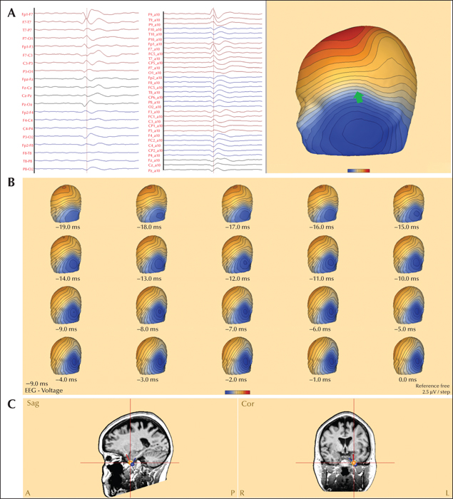
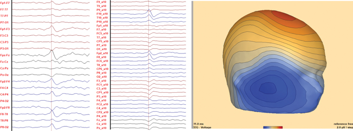
Figure 8
Left temporal anterior basal. (A) Maximum negativity: left anterior-inferior temporal (F7 in double banana; F9 earlier than F7 in the extended array). Maximum positivity: F4 (earliest positivity: Pz). The green arrow in the voltage map shows the location of the steepest voltage gradient at -17 ms. This voltage distribution and the vertical orientation indicate a source in the anterior-basal region of the left temporal lobe. (B) Sequential voltage maps show changes in time throughout the ascending slope of the spike. At onset (-19 ms), a vertical orientation is observed, as described in the previous figure. This gradually evolves into a more radial orientation at peak (0 ms), due to the propagation of the activity to the lateral part of the left anterior temporal lobe. (C) Equivalent current dipole modelling indicates an onset source in the anterior-basal part of the left temporal lobe (red dipole) with following propagation to polar-lateral areas (blue).Intracranial recordings (SEEG) demonstrated the irritative zone in the left temporal lobe, with IEDs in the basal and lateral part more frequent than in the mesial part. The patient underwent left anterior temporal lobectomy and achieved Engel Class 1 at 27 months after operation.
Figure 8 -
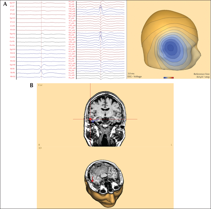
Figure 9
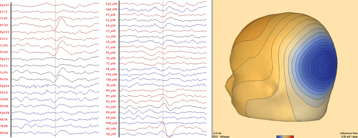
Right temporal lateral. (A) Maximum negativity: right temporal (T8), surrounded by widely distributed, low-amplitude positivity, as shown in the common average montage. This voltage distribution indicates a radial orientation, hence the source is under the maximum negativity. (B) Equivalent current dipole modelling indicates a source in the right lateral temporal region. Previously, the patient underwent selective amygdalo-hippocampectomy, which did not render the patient seizure-free. The second operation removed the temporal lateral tissue including the source, and the patient became seizure-free (Engel Class 1 at 36 months after operation).
Figure 9 -
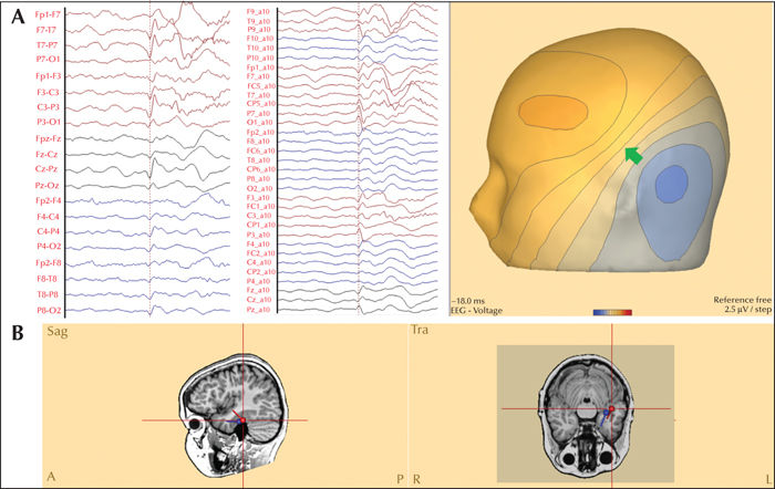
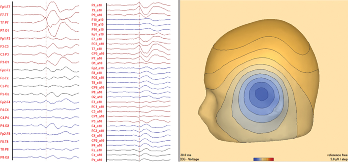
Figure 10
Left temporal basal. (A) Maximum negativity: left posterior temporal (T7) and occipital (O1). Maximum positivity: left frontal (F3). The green arrow in the voltage map shows the location of the steepest voltage gradient. This voltage distribution and the close-to-vertical orientation indicate a source in the basal part of the left temporal lobe, anterior to the peak negativity. (B) Equivalent current dipole indicating a source in the posterior basal part of the left temporal lobe.The patient underwent resection of the temporal pole, amygdala and the anterior part of caput hippocampi without resecting the source. The patient is not seizure-free (six months post-operation).
Figure 10 -
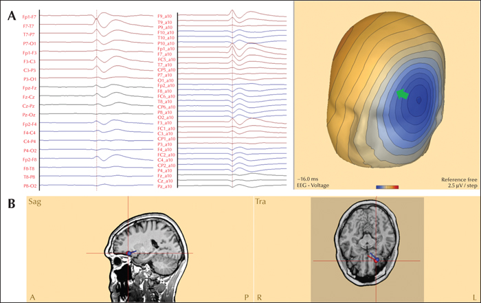
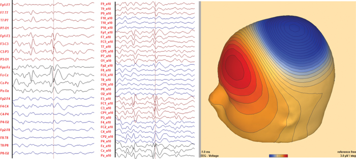
Figure 11
Left orbito-frontal. (A) Maximum negativity: left fronto-temporal (F7). Maximum positivity: right fronto-central (F4-C4). The green arrow in the voltage map shows the location of the steepest voltage gradient. This helps to distinguish between a frontal and temporal source, indicating that the generator is in the anterior-basal area of the left frontal lobe (orbito-frontal cortex). (B) Equivalent current dipole indicating a source in the left orbito-frontal cortex, confirmed by electrocorticography.
Figure 11 -
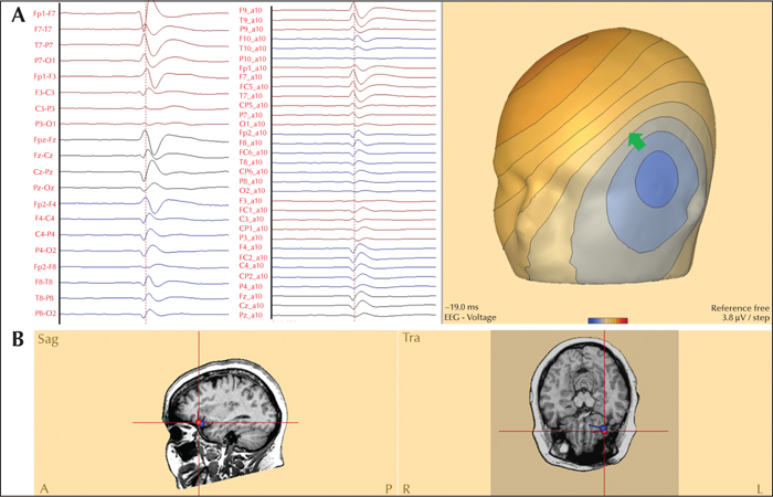
Figure 12
Left frontal operculum. (A) Maximum negativity: left fronto-temporal (F7-T7). Maximum positivity: right fronto-central (FC2). The green arrow in the voltage map shows the location of the steepest voltage gradient. This and the anterior positivity help to distinguish between a frontal and temporal source, indicating that the generator is in the superior wall of the anterior Sylvian fissure (anterior frontal operculum). (B) Equivalent current dipole modelling indicates a source in the anterior part of the left frontal operculum, where the MRI showed focal cortical dysplasia.
Figure 12 -
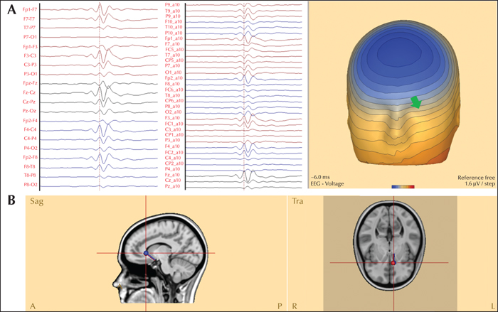
Figure 13
Left frontal-mesial (pre-supplementary motor area). (A) Maximum negativity: bi-frontal and midline (Fz). Maximum positivity: left inferior temporal (F9-P9). The green arrow in the voltage map shows the location of the steepest voltage gradient. This and the location of the positivity help to lateralize the source to the left hemisphere, as indicated by the green arrow. (B) Equivalent current dipole modelling indicates a source in the left mesial frontal lobe. The patient had focal cortical dysplasia in the left pre-SMA area.
Figure 13 -
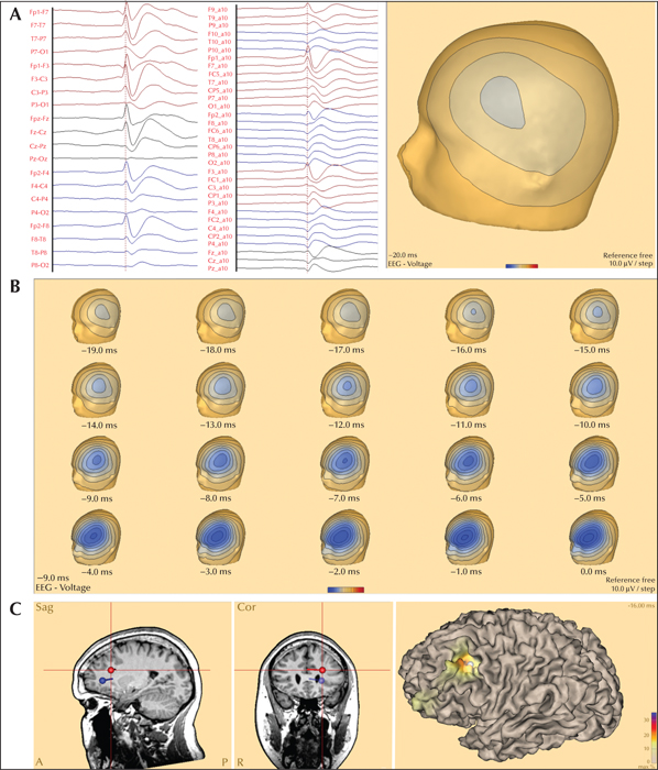
Figure 14
Left frontal-lateral. (A) Maximum negativity: left frontal (F3). Widely distributed, low-amplitude positivity, mainly in the right fronto-central area. This suggests a radial orientation, hence the source is under the peak negativity in the left frontal lobe. (B) Sequential voltage maps showing changes in the voltage map over time through the ascending slope of the spike. At onset (-19 ms), the maximum negativity is in the left frontal area, as described in the previous figure. This gradually evolves into a voltage distribution with maximum negativity in the fronto-polar area at the peak of the spike (0 ms), due to the propagation of the activity to the more anterior parts in the frontal lobe. (C) Equivalent current dipole and distributed source models show the onset (red dipole) in the lateral convexity of the left frontal lobe with following propagation to more anterior left frontal areas. The focal cortical dysplasia in this patient was in the same sub-lobar region as the onset.
Figure 14 -
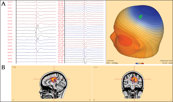
Figure 15
Left gyrus cinguli, posterior. (A) In the classic “double-banana”, the maximum negativity (phase reversal) is in the midline (Cz) and on both parasagittal chains (C3-P3 and C4-P4). Although this suggests a generator in the centro-parietal midline, the side is unclear. The voltage map shows maximum negativity at the vertex (Cz-Pz), and a positive pole, with maximum positivity located at F9. This voltage distribution indicates an oblique orientation (negative pole much stronger than positive pole) of the source. The green arrow in the voltage map shows the location of the steepest voltage gradient. This helps to lateralize the source to the left hemisphere. The depth of the left centro-parietal source can be difficult to estimate from the voltage maps. (B) Equivalent current dipole and distributed source model indicating a source in the posterior part of the left cingulate gyrus, confirmed by intracranial recordings (SEEG).
Figure 15 -
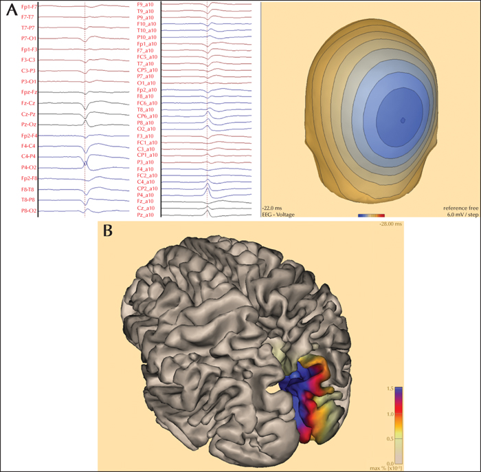
Figure 16
Right parieto-occipital, mesial / parasagittal. (A) Maximum negativity: parietal, midline and right parasagittal (Pz, P4). Widely distributed, low-amplitude positivity, indicating a radial orientation of the source. Hence, the source is under the peak negativity. (B) Source imaging showing the mesial and parasagittal part of the right parietal lobe, in the same sub-lobar region as focal cortical dysplasia.
Figure 16 -

Figure 17
Right occipital – large network: mesial-lateral. (A) At the peak of the spike, the montages show maximum negativity over the right parieto-temporal area (P4, P8). The voltage map (head seen from behind) at the onset of the spike (start of the ascending slope) shows maximum negativity over the left parieto-occipital area, and a stronger positive pole in the right parieto-temporal area. This suggests an oblique orientation with the generator closer to the positive pole. The green arrow in the voltage map shows the location of the steepest voltage gradient. This helps to lateralize the source to the right hemisphere – mesial part of the occipital lobe. (B) Sequential voltage maps through the ascending slope of the spike show the changes of topography over time. At onset (-33 ms), the maximum negativity is over the left parieto-occipital area, as described in the previous figure. This gradually evolves into a voltage distribution with maximum negativity in the right occipital area (-15 ms) and then right parieto-temporal area at the peak of the spike. (C) Equivalent current dipoles show the onset (red dipole) in the mesial part of the right occipital lobe and propagation to the lateral convexity (blue dipole). This widely distributed network in the posterior part of the right hemisphere was confirmed by intracranial recordings (SEEG).
Figure 17 -
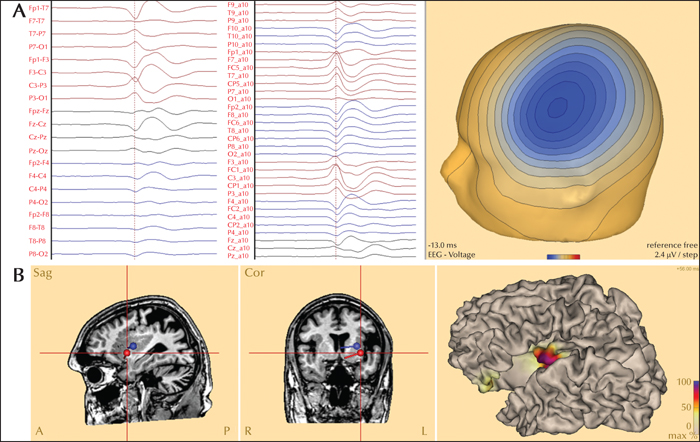
Figure 18
Left insula. (A) Maximum negativity: left central-temporal area (C3, T7). The widely distributed, low-amplitude positivity suggests a radial orientation. Hence, the source is under the peak negativity in the left centro-temporal area. (B) Equivalent current dipole and distributed source models show a generator in the left insula, where the polymicrogyria was located.
Figure 18 -
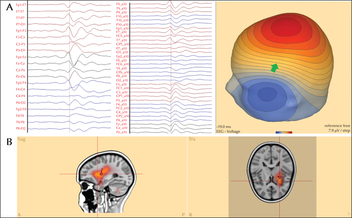
Figure 19
Left frontal operculum. (A) Negative pole over left fronto-temporal area (F7), positive pole of similar magnitude at Cz. This suggests a tangential orientation. The green arrow in the voltage maps shows the steepest voltage gradient, indicating a source in the frontal operculum considering the distance and similar magnitude of both poles. In the case of a temporal-polar spike, the negative pole ought to be stronger in comparison to the positive pole. (B) Equivalent current dipole and distributed source models showing a source in the left frontal operculum and insula, confirmed by intracranial recordings (SEEG).
Figure 19 -

Figure 20
Left posterior insula. (A) Maximum negativity: left centro-temporal area (C3-T7). Clear positive pole with maximum at Pz. The stronger negative pole suggests an oblique orientation with the source closer to the negative pole. The green arrow in the voltage maps shows the steepest voltage gradient, suggesting a source in the posterior part of the left insula. Here again, the relatively strong positive pole and its large distance from the negative pole suggest a deeper source than that of the central operculum. (B) Equivalent current dipole and distributed source models showing a generator in the posterior part of the left insula, co-localized with hypometabolism on FDG-PET.
Figure 20
- Mots-clés : atlas, interictal epileptiform discharges, localization, source, topographic maps, voltage maps
- DOI : 10.1684/epd.2021.1396
- Page(s) : 229-48
- Année de parution : 2022
Describing the location of EEG abnormalities, such as interictal epileptiform discharges, is an important step in the interpretation of EEG recordings and has clinical relevance, as it is expected to point out the region of the brain generating these abnormal signals. Traditionally, the location is reported by specifying the area on the scalp where maximum negativity is located. However, this only reflects the correct localization in the brain when the cortical generator is located on the convexity (radial orientation). When the cortical generator is in the wall of a sulcus (tangential orientation), due to current flow (volume conduction), the maximum negativity is not over the generator, but at a distance from it. Voltage maps are widely available in most EEG reader software programs. Simple rules for reading voltage maps help to estimate the orientation and location of the source in the brain, avoiding false lateralization and false localization. In this seminar in epileptology, using a didactic approach, we explain how to read voltage maps and provide an atlas of voltage maps.
 Cette œuvre est mise à disposition selon les termes de la
Licence Creative Commons Attribution - ShareAlike 3.0 International
Cette œuvre est mise à disposition selon les termes de la
Licence Creative Commons Attribution - ShareAlike 3.0 International